PCR vs qPCR vs RT-PCR vs Digital PCR: What Each One Measures

PCR, qPCR, RT-PCR, RT-qPCR, digital PCR. The names differ by a letter or two, they turn up in the same papers, and a methods section will happily use three of them in one paragraph. Ask a room of students what "RT" stands for and you will get two confident answers, both in use, with different meanings.

The confusion matters because these are not five versions of one experiment. They answer different questions. One tells you whether a piece of DNA is present. One tells you how much of it there was before you started. One counts molecules one by one. Choosing the wrong method means answering a question nobody asked.

This guide sorts them out by asking the same thing of each method: what does the instrument physically measure, and what does that let you claim? By the end you will be able to:

• decode any of the names on sight, and say what each letter adds
• explain why a gel band cannot tell you how much template you started with
• read a Cq value and turn a difference in Cq into a fold change
• work through the delta-delta-Cq calculation by hand, and say what it assumes
• explain how digital PCR counts molecules without a standard curve
• pick the right method for a question, and name the controls it needs

You need no background beyond knowing that DNA is double-stranded and that RNA is copied from it. The qPCR curves in the figures are real, taken from a published dilution series of 375 reactions.

Six names, two choices

Every name in this family is built from two independent choices: what you start from, and how you read the result.

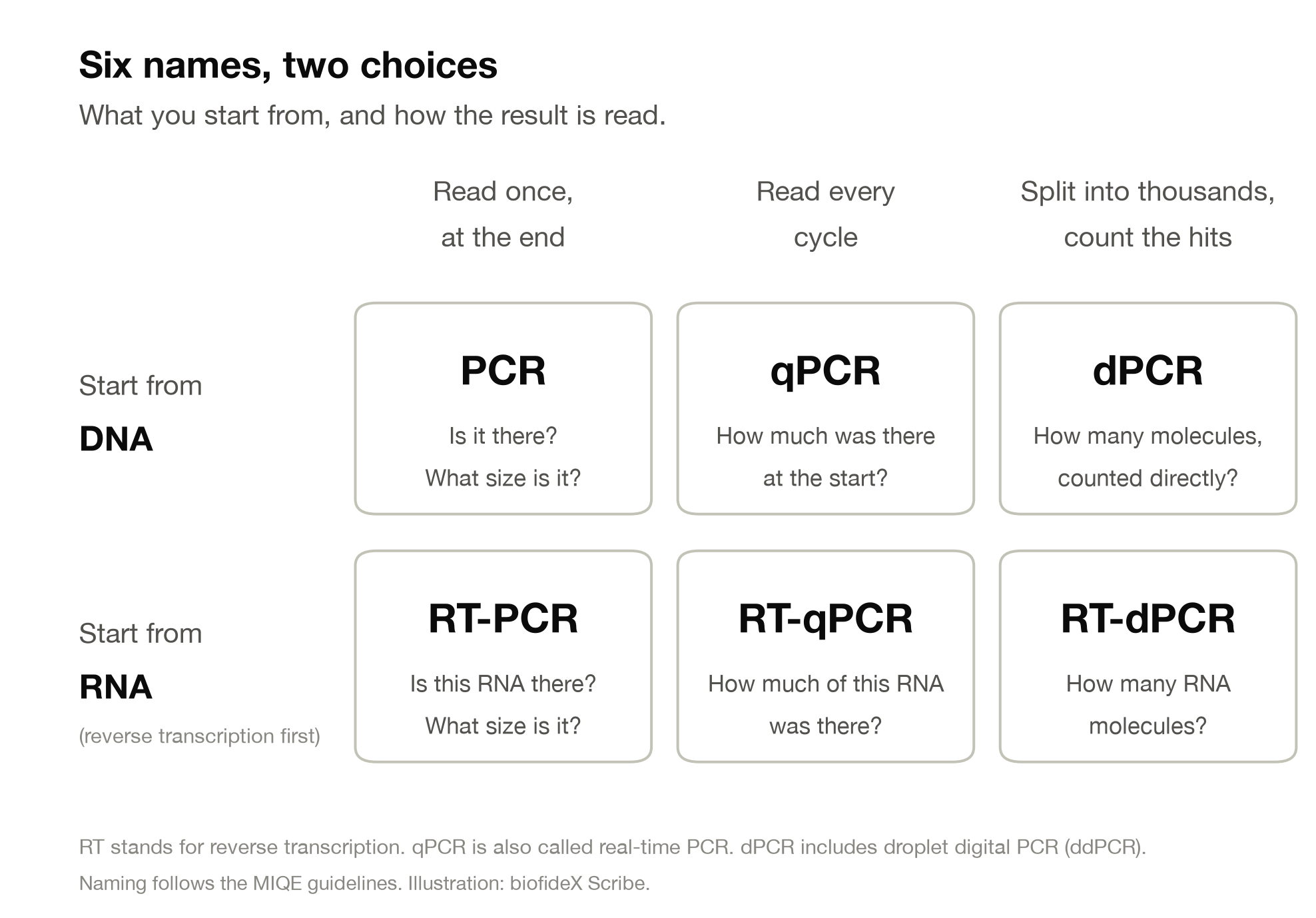
Choice 1: what goes in. PCR copies DNA. If your sample is RNA, such as a messenger RNA or the genome of an RNA virus, it must first be copied into DNA. That step is called reverse transcription, and it adds the prefix RT-.

Choice 2: how the result is read. There are three options:

• Once, at the end. Run all the cycles, then look at the product. This adds no letter. It is often called conventional or end-point PCR.
• Every cycle. Measure the product after each cycle while the reaction runs. This is quantitative PCR, written q, and also called real-time PCR.
• By counting. Split the sample into thousands of tiny separate reactions and count how many of them light up. This is digital PCR, written d. Droplet digital PCR (ddPCR) is one way of doing the splitting.

Two starting materials times three read-outs gives the six names in Figure 1. Once you see the grid, a name like RT-qPCR stops being jargon: it starts from RNA and is read every cycle.

The two letters that cause the trouble

"RT" is used in the literature for both "reverse transcription" and "real-time". So "RT-PCR" in one paper means PCR that starts from RNA, and in another it means PCR that is watched as it runs.

The MIQE guidelines, the reporting standard for this field, settle the matter. RT means reverse transcription and nothing else. Real-time PCR is written qPCR. The two together are RT-qPCR. This article follows that convention.

Older papers and many kit manuals do not, so check which meaning is intended.

PCR in one minute

PCR is a chain reaction that copies one chosen stretch of DNA, and in each cycle the number of copies roughly doubles.

The tube holds the sample DNA, two short primers that mark the ends of the target, loose DNA building blocks, and a heat-stable polymerase enzyme. A machine then cycles the temperature through three steps:

1. 1Denature, at about 95 °C. The two strands of the DNA come apart.
2. 2Anneal, at about 50 to 65 °C. The primers stick to their matching sequences.
3. 3Extend, at about 72 °C. The polymerase builds a new strand from each primer.

One round turns each target molecule into two. Thirty rounds turn one molecule into 2³⁰, which is about a billion.

That doubling cannot last. Primers and building blocks get used up, the enzyme wears out, and the product strands start pairing with each other instead of with primers. The reaction slows and flattens.

So every PCR passes through three phases:

• Baseline. The product is doubling, but there is too little of it to see.
• Exponential. The product is visible and still doubling cleanly.
• Plateau. The reagents are running out and the amount levels off.

This is the key to the rest of the article. The three read-outs in Figure 1 look at different parts of the same reaction. End-point PCR looks at the plateau. qPCR looks at the moment the exponential phase rises out of the baseline. Digital PCR also looks at the end, but asks only a yes-or-no question of each tiny reaction.

End-point PCR: is it there?

End-point PCR runs all its cycles first and looks at the product afterwards. It answers yes-or-no questions well and how-much questions badly.

What it measures

After 25 to 40 cycles, the product is usually run on an agarose gel with a dye that binds DNA. Fragments travel through the gel according to their length, and a band appears wherever product has gathered.

So the read-out is a band: whether it is there, and where it sits. That answers several useful questions:

• Is the target sequence present? This covers genotyping, checking a clone, confirming a knockout and detecting a pathogen.
• Is the product the expected length? Insertions, deletions and alternative splice forms all change it.
• Can I have more of this DNA? The product itself is often the goal, for cloning or sequencing.

Why the band cannot tell you how much you started with

It is tempting to read a brighter band as more starting material. Figure 2 shows why that fails. It holds 375 real reactions that began with 15, 150, 1,500 or 15,000 copies of the same DNA, and it tracks the amount of product through all 45 cycles.

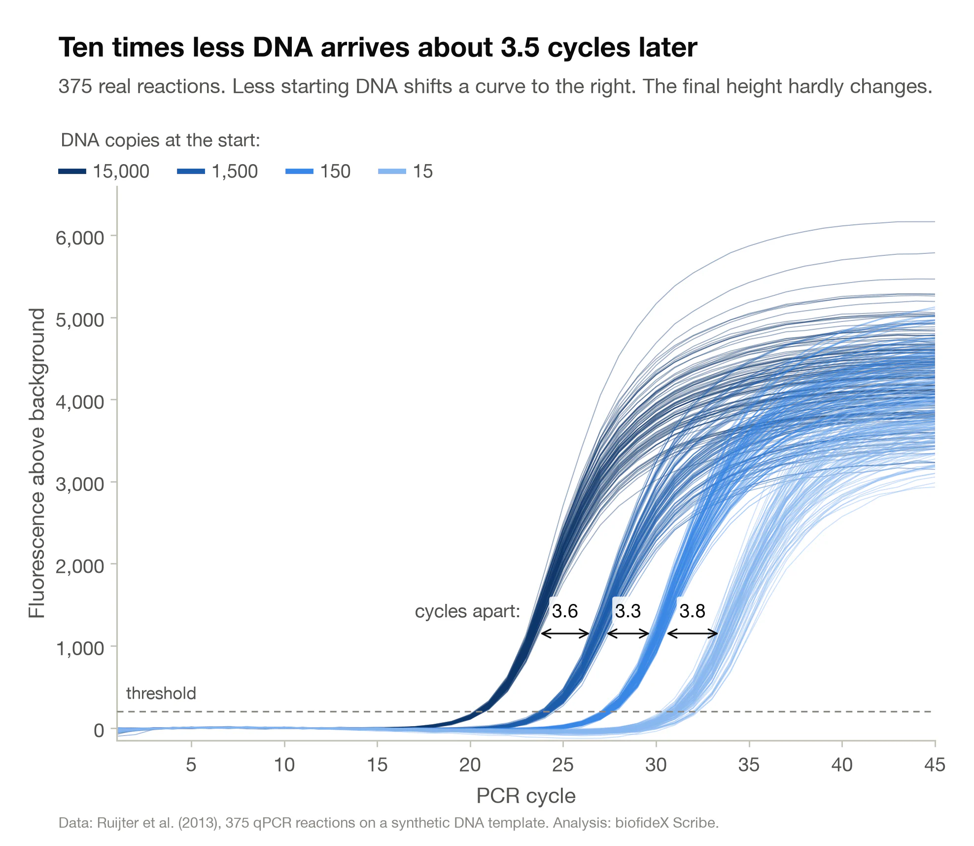
Follow any curve to the right-hand edge. That final height is all that end-point PCR sees.

• The reactions that began with 15,000 copies finish at an average signal of 4,467 units.
• The reactions that began with 15 copies finish at 3,720.

A thousandfold difference at the start has become a 20% difference at the end. That is smaller than the scatter between identical tubes: within the 15-copy group alone, single reactions finished anywhere from 2,934 to 4,760.

The two middle groups are even in the wrong order. The 150-copy reactions finish higher, at 4,275, than the 1,500-copy reactions, at 4,017.

The reason is the plateau. Its height reflects what ran out, not what went in. Every reaction climbs until it hits roughly the same ceiling, and by then the starting amount has been forgotten.

When it is the right tool

End-point PCR is cheap, quick to set up and needs no fluorescence instrument. For presence, absence and size it remains the sensible choice. It is the wrong tool the moment the question contains the words "how much".

qPCR: how much was there at the start?

qPCR measures the product after every cycle. That lets it use the one part of the reaction that still remembers the starting amount: the moment the curve takes off.

What it measures

The reaction contains a fluorescent reporter whose signal grows with the amount of product. The instrument reads that signal at every cycle and draws curves like those in Figure 2.

For the first cycles nothing shows. The product is doubling, but below what the detector can see. Then the signal rises out of the background. The more template a tube began with, the fewer doublings it needs to get there, so the earlier it rises.

The instrument reduces each curve to one number: the cycle at which it crosses a fixed threshold. This is the quantification cycle, or Cq. You will also meet Ct (threshold cycle) and Cp (crossing point). They are the same thing, and the MIQE guidelines recommend Cq.

How to read a Cq value

Two rules cover most of it.

1. 1A lower Cq means more template. This runs against instinct, so say it twice.
2. 2Cq is a logarithm. Each cycle is one doubling, so a difference in Cq is a ratio, not an amount.

difference in Cq     difference in starting amount
      1                       2 times
      2                       4 times
      3.3                    10 times
      5                      32 times
      6.6                   100 times
     10                   1,024 times

Those figures assume perfect doubling. In Figure 2 the four groups cross the threshold at an average Cq of 20.5, 24.1, 27.3 and 31.1. Each tenfold drop in template costs 3.3 to 3.8 cycles.

The standard curve and efficiency

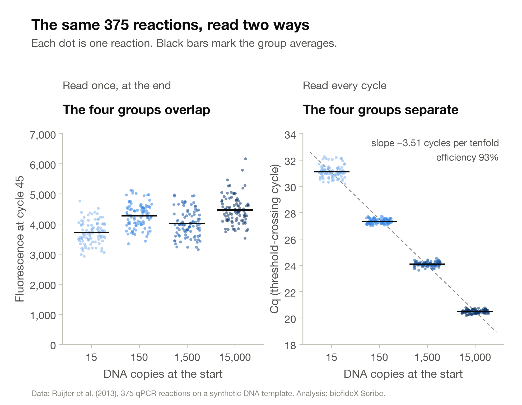
The right-hand panel of Figure 3 is a standard curve: known amounts along the bottom, Cq up the side. It does two jobs.

It turns a Cq into a copy number. Run an unknown sample next to the standards, read its Cq across to the line and down to the axis. This is called absolute quantification.

It tests the assay. The slope of the line says how well the reaction doubles. Perfect doubling gives a slope of −3.32 cycles per tenfold. The usual conversion is:

efficiency = 10^(-1/slope) - 1

slope -3.32   ->  100%   every cycle doubles the product
slope -3.51   ->   93%   the real data in Figure 3
slope -3.60   ->   90%

Our real dataset has a slope of −3.51, an efficiency of 93%. Each cycle multiplies the product by 1.93 and not by 2. That is a perfectly respectable assay. Most labs accept 90% to 110%.

An efficiency above 100% is not a better reaction, since nothing can more than double. It usually points to a problem in the dilution series, such as pipetting error or something in the concentrated samples that slows the reaction.

Where the fluorescence comes from

There are two main chemistries.

• DNA-binding dyes, such as SYBR Green. These glow when bound to double-stranded DNA. They are cheap and work with any primer pair. But they light up any double-stranded DNA, including the wrong product. So a dye-based run ends with a melt curve: the product is heated slowly, and a single sharp drop in fluorescence indicates a single product.
• Hydrolysis probes, such as TaqMan probes. A third short piece of DNA sits inside the target, carrying a reporter and a quencher. The polymerase destroys the probe as it copies, which frees the reporter. Signal comes only from the intended target, and probes of different colours let you measure several targets in one tube. They cost more.

Where qPCR runs out of road

Look again at the right-hand panel of Figure 3. The clusters are tight at 15,000 copies and loose at 15.

• At 15,000 copies, the 94 identical reactions span 0.6 cycles.
• At 15 copies, they span 2.1 cycles, which is about a fourfold range in apparent amount.

The instrument is not at fault. A tube meant to receive 15 molecules gets 11 by chance, and its neighbour gets 19. We checked: the scatter in the 15-copy group matches what random sampling of about 15 molecules predicts.

Extend the line in Figure 3 down to a single copy and it reaches a Cq of about 35. In this assay, a signal later than that corresponds to less than one molecule. The exact number differs from assay to assay, but the lesson holds everywhere: late Cq values need more replicates and more suspicion.

Starting from RNA: what "RT" adds

Reverse transcription copies RNA into DNA, so that PCR has something it can work on.

The polymerases used in PCR copy DNA and nothing else. Yet many of the most interesting questions are about RNA: which genes a cell has switched on, or how much of an RNA virus a patient carries. A reverse transcriptase, an enzyme borrowed from retroviruses, bridges the gap. It reads an RNA molecule and builds the matching strand of DNA, called complementary DNA or cDNA.

After that, everything in the earlier sections applies unchanged. RT in front of end-point PCR gives RT-PCR. RT in front of qPCR gives RT-qPCR, the standard way to measure gene expression.

One step or two

• Two-step. Reverse transcription is done first, in its own tube. A portion of the cDNA then goes into each PCR. The cDNA can be stored and used for many different genes, which suits gene expression studies.
• One-step. Both enzymes share one tube, so RNA goes in and a result comes out. There is less handling and less chance of contamination, which suits diagnostic testing. Each reaction uses up some of the RNA.

How the reverse transcription is primed

The enzyme needs a primer to start from, and the choice shapes what gets copied.

• Oligo(dT) binds the poly(A) tail found on most messenger RNAs, so it favours them.
• Random hexamers bind anywhere, so they copy all kinds of RNA.
• Gene-specific primers copy only the target, and are the usual choice in one-step reactions.

Pick one and keep it for the whole study. Results made with different priming methods are not comparable.

The weakest link

Reverse transcription does not convert every RNA molecule, and how many it converts varies with the enzyme, the priming, the quality of the RNA and whatever was carried over from the extraction.

So an RT-qPCR result is never "how much RNA was in the cell". It is "how much RNA survived extraction and was converted". The practical defence is consistency: the same kit, the same amount of input RNA and the same protocol for every sample you intend to compare.

The control that RNA work demands

RNA preparations carry traces of genomic DNA, and PCR cannot tell cDNA from genomic DNA. A no-RT control exposes the problem. It contains everything except the reverse transcriptase, so any signal in it comes from contaminating DNA.

Two further defences are common: treating the RNA with DNase, and designing primers that span the junction between two exons, a sequence that exists in spliced RNA and not in the genome.

Why the COVID test had two RTs in its name

The test much of the world took in 2020 is a good exercise in decoding. The virus has an RNA genome, so the test begins with reverse transcription. The result is read every cycle, so it is real-time PCR.

The US Centers for Disease Control and Prevention described its assay as a "Real-Time Reverse Transcription PCR Panel": both meanings of RT in one name. In the convention used here, it is simply RT-qPCR.

The "Ct values" that reached the news were Cq values. A lower one meant more viral RNA in the swab. And because a Cq has no meaning outside its own assay, values from different laboratories could not fairly be compared.

Relative quantification: the delta-delta-Cq method

Most gene expression experiments do not need copy numbers. They ask how many times higher or lower a gene is in one condition than in another. The delta-delta-Cq method answers that with four Cq values and no standard curve. You will also see it written ΔΔCt or 2^−ΔΔCt.

The idea

The method makes two corrections, one after the other.

1. 1Correct for how much material went into each tube. Measure a reference gene in the same sample and subtract its Cq. This gives ΔCq.
2. 2Compare the two conditions. Subtract the control's ΔCq from the treated sample's. This gives ΔΔCq.

A worked example

Suppose you treat cells with a drug and measure a gene called IL6, plus a reference gene that the drug should not affect. These are the average Cq values:

                 IL6    reference    dCq = IL6 - reference
control cells    27.0     18.0             9.0
treated cells    24.4     18.2             6.2

ddCq        = 6.2 - 9.0 = -2.8
fold change = 2^(-ddCq) = 2^2.8 = 7.0

Step by step:

1. 1For each sample, subtract the reference Cq from the IL6 Cq. Control: 27.0 − 18.0 = 9.0. Treated: 24.4 − 18.2 = 6.2. A smaller ΔCq means more IL6 relative to the reference.
2. 2Subtract the control ΔCq from the treated one: 6.2 − 9.0 = −2.8.
3. 3Raise 2 to the power of minus that number: 2^2.8 is about 7.

IL6 is about seven times higher in the treated cells.

Notice what the reference gene did. The raw IL6 Cq fell by 2.6 cycles, which on its own suggests a sixfold rise. But the treated sample's reference came up 0.2 cycles late, a sign that slightly less material went into that tube. Allowing for that lifts the answer to sevenfold.

What the method quietly assumes

The calculation is simple because it takes three things for granted.

That both assays double perfectly. The 2 in the formula is an efficiency of 100%. Suppose both assays really ran at 93%, like the data in Figure 3. Each cycle then multiplies by 1.93, and the true change is 1.93^2.8, about 6.3-fold. The formula has overstated it by 11%.

The error grows with the gap. Across 8 cycles, the formula says 256-fold where the truth is about 190-fold, an overstatement of 35%. When efficiencies are known, the Pfaffl method uses each assay's measured value in place of 2.

That the reference gene does not change. Favourites such as GAPDH and beta-actin do change under some treatments. If the reference moves, part of your fold change is an artefact. The defence is to test candidate reference genes in your own system and to average two or three stable ones.

That the averages tell the whole story. One cycle is a factor of two, so small scatter matters. A difference of 0.3 cycles between replicate tubes is already a 23% difference in amount. Report the spread across biological replicates, and run statistics on the ΔCq values, which are on a log scale, before converting to fold change.

Digital PCR: count the molecules

Digital PCR replaces one measurement with thousands of yes-or-no answers, and works out a count of molecules from the share that say yes.

What it measures

The sample is split into a very large number of tiny partitions before any cycling begins. These are droplets in oil or wells on a chip, and one widely used system makes about 20,000 droplets per sample. The sample is dilute enough that each partition holds zero, one or a few target molecules.

Every partition is then run to the end, like a miniature end-point PCR. A partition that held at least one target molecule lights up. A partition that held none stays dark. The instrument counts the two kinds.

Notice what has disappeared: there is no Cq, no standard curve and no need for perfect doubling. A partition only has to cross the line between dark and lit.

Why you cannot simply count the lit partitions

Molecules land in partitions at random, so some partitions receive two or more and still count only once. The share of partitions left empty reveals how crowded things were, through one line of arithmetic:

copies per partition = -ln(1 - share of partitions lit)
total copies         = copies per partition x number of partitions

Here is a worked example. Of 20,000 partitions, 6,000 light up.

1. 1The share lit is 6,000 ÷ 20,000 = 0.30.
2. 2Copies per partition = −ln(1 − 0.30) = −ln(0.70) = 0.357.
3. 3Total copies = 0.357 × 20,000 = 7,133.

Counting lit partitions alone would have given 6,000 and missed 16% of the molecules. The step is called the Poisson correction, after the statistics of random scattering.

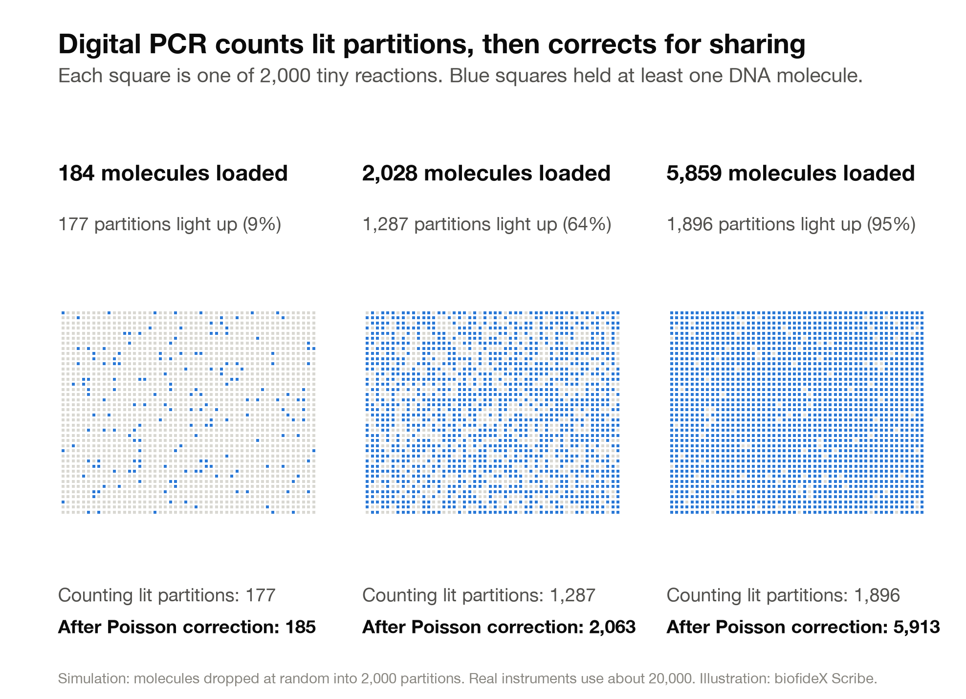
Figure 4 shows the correction at work. In the middle panel, 2,028 molecules lit only 1,287 partitions, and the correction returns 2,063. On the left, where partitions are sparse, the raw count of 177 is already close to the truth of 184.

Its limits are visible in the same figure

In the right-hand panel, 95% of partitions are lit. The estimate now rests entirely on the 104 that stayed dark, and a handful more or fewer by chance would swing the answer. Load more still and every partition lights up, at which point the instrument can say only "a lot". The remedy is to dilute and run again.

At the other extreme, a sample with ten target molecules gives about ten lit partitions, and counting ten of anything is imprecise.

So digital PCR has a narrower working range than qPCR, set by the number of partitions. qPCR comfortably spans a millionfold range in one run.

What it is good at

• Absolute counts. The answer comes as copies per microlitre, with no standard curve to prepare or to get wrong.
• Small differences. Telling two copies of a gene from three is a 1.5-fold difference. In qPCR that is 0.58 of a cycle, close to the noise. Counting resolves it.
• Rare variants. A mutant sequence hidden among thousands of normal copies ends up alone in its own partitions, where it is easy to see. This is the basis of many tests for tumour DNA in blood.
• Difficult samples. Substances that slow a reaction shift a Cq, but a slowed partition still ends up lit. Digital PCR is more tolerant of such inhibitors, though not immune.

What it costs

Instruments and consumables cost more per sample, fewer samples fit in a run, and the method still depends on good primers and probes. A partition that lights up for the wrong reason is counted as a molecule.

Which one do you need?

Start from the question you are asking, not from the instrument that happens to be free. If your sample is RNA, add reverse transcription in front of whichever method you land on.

• "Is this sequence here at all?" Use end-point PCR. This covers genotyping, clone checks and simple pathogen detection.
• "Is the product the right length, or can I have more of it?" Use end-point PCR.
• "Does this gene's expression change between my conditions?" Use RT-qPCR with the delta-delta-Cq method and reference genes you have tested.
• "How many copies are in my sample?" Use qPCR with a standard curve, or digital PCR if you would rather not depend on one.
• "Is this difference real if it is under twofold?" Use digital PCR. Gene copy number is the classic case.
• "Is a rare variant hiding among a great excess of normal sequence?" Use digital PCR.
• "I have hundreds of samples covering a huge range of concentrations." Use qPCR. Viral load testing is the classic case.
• "My samples are dirty: soil, stool, wastewater." Digital PCR tolerates inhibitors better. Diluting the sample and using qPCR is the cheaper first try.

The three read-outs side by side:

            end-point PCR     qPCR                digital PCR

reads       a band, at the    fluorescence,       lit or dark,
            end               every cycle         per partition

gives       present or not,   Cq: a relative      a count of
            and length        amount, or copies   molecules
                              via standards

best for    presence, size,   expression change,  small differences,
            making product    viral load, many    rare variants,
                              samples             absolute counts

weak at     amounts           differences under   very wide ranges,
                              twofold, very few   cost per sample
                              copies

The methods are not rivals. A typical project uses end-point PCR to check its constructs, RT-qPCR to measure expression, and digital PCR only where a small difference or an absolute number really matters.

Mistakes that ruin a run

PCR is sensitive enough to amplify a single molecule, which means it will also amplify a single molecule of the wrong thing. These nine checks separate a result from an artefact.

1. 1Running without a no-template control. This is a reaction with water in place of the sample. Any signal in it comes from contamination or from primers sticking to each other. Include one for every assay in every run.
2. 2Running RNA work without a no-RT control. Without it you cannot show that your signal came from RNA and not from stray genomic DNA.
3. 3Trusting a reference gene you never tested. If the reference shifts with your treatment, every fold change you report is shifted with it.
4. 4Assuming 100% efficiency. Run a dilution series for each new primer pair and calculate the slope before you rely on it.
5. 5Skipping the melt curve in a dye-based run. A second peak means a second product, and the dye counted both.
6. 6Reading too much into a late Cq. Scatter between replicates, primer artefacts and contamination all live at the late end of the run. In our data, a single molecule would sit near Cq 35.
7. 7Comparing raw Cq values between runs, assays or labs. Compare within a run, or through a standard curve or a shared calibrator sample.
8. 8Carrying product back into the set-up area. A finished reaction tube holds billions of copies of your target. Open it near tomorrow's reagents and every future run is contaminated. Keep set-up and analysis in separate places with separate pipettes.
9. 9Mistaking technical replicates for biological ones. Three wells filled from one sample measure your pipetting. Only separate animals, patients or cultures measure the biology.

What to take away

The names differ by a letter or two, but the measurements differ in kind.

• The name is a recipe. RT- means it starts from RNA. A q means it is read every cycle. A d means it is split up and counted.
• End-point PCR reads the plateau. By then the reaction has forgotten how much it started with, so use it for presence and size.
• qPCR reads the take-off. A lower Cq means more template, each cycle is a doubling, and about 3.3 cycles is tenfold.
• Delta-delta-Cq turns four Cq values into a fold change. Trust the result exactly as far as you trust the efficiency and the reference gene behind it.
• Digital PCR counts. It is the tool for small differences, rare targets and absolute numbers, within a narrower range.
• Every method needs its controls. A no-template control always, and a no-RT control whenever RNA is involved.

The next time a methods section says "RT-PCR", ask the two decoding questions. Was the starting material RNA or DNA? And was the result read once at the end, every cycle, or by counting? The answers tell you what the authors could have measured, and what they could not.

Sources and methods

How the figures were made

Figures 2 and 3 use a public dataset from Ruijter and colleagues (2013): four tenfold dilutions of a synthetic copy of part of the human MYCN gene, with 94 replicate reactions at each, run with SYBR Green dye on a Bio-Rad CFX384 instrument. We took it from the R package qpcR, version 1.4-2, where it is called dil4reps94. It holds 375 reactions, because one is missing from one group.

For each reaction we removed its own background by fitting a straight line to cycles 3 to 12 and subtracting it. The Cq is the fractional cycle at which the corrected curve crossed 200 fluorescence units, found by straight-line interpolation between two cycles.

The package describes the four groups as 15 to 15,000 copies. In the file, the group labels run opposite to the order in which the curves rise. More template has to amplify earlier, so we assigned the copy numbers by that order. The scatter between replicates supports the assignment: in the last group to rise, it matches random sampling of about 15 molecules.

Figure 4 is a simulation in which molecules were assigned at random to 2,000 partitions. Figure 1 is an illustration. The delta-delta-Cq example uses invented round numbers. The analysis was run in October 2026.

Further reading

Naming and reporting. Bustin SA and colleagues (2009). The MIQE guidelines: minimum information for publication of quantitative real-time PCR experiments. Clinical Chemistry 55(4): 611-622. The 2025 revision is MIQE 2.0, Clinical Chemistry 71(6): 634-651.

The delta-delta-Cq method. Livak KJ, Schmittgen TD (2001). Analysis of relative gene expression data using real-time quantitative PCR and the 2(-Delta Delta C(T)) method. Methods 25(4): 402-408.

Correcting for efficiency. Pfaffl MW (2001). A new mathematical model for relative quantification in real-time RT-PCR. Nucleic Acids Research 29(9): e45.

Choosing reference genes. Vandesompele J and colleagues (2002). Accurate normalization of real-time quantitative RT-PCR data by geometric averaging of multiple internal control genes. Genome Biology 3(7): research0034.

The idea of digital PCR. Vogelstein B, Kinzler KW (1999). Digital PCR. Proceedings of the National Academy of Sciences 96(16): 9236-9241.

Droplet digital PCR. Hindson BJ and colleagues (2011). High-throughput droplet digital PCR system for absolute quantitation of DNA copy number. Analytical Chemistry 83(22): 8604-8610.

Reporting digital PCR. The dMIQE Group, Huggett JF (2020). The digital MIQE guidelines update: minimum information for publication of quantitative digital PCR experiments for 2020. Clinical Chemistry 66(8): 1012-1029.

The dilution dataset. Ruijter JM and colleagues (2013). Evaluation of qPCR curve analysis methods for reliable biomarker discovery: bias, resolution, precision, and implications. Methods 59(1): 32-46.

The COVID assay. Lu X and colleagues (2020). US CDC real-time reverse transcription PCR panel for detection of severe acute respiratory syndrome coronavirus 2. Emerging Infectious Diseases 26(8): 1654-1665.